Adedeji Awolesi

Cost visibility is the foundation of the FinOps Inform stage, enabling organizations to understand where cloud spending occurs and who’s responsible for it. In this hands-on guide, we’ll build a complete cost visibility solution on AWS by deploying tagged resources with Terraform and creating department-specific dashboards in AWS Cost Explorer.

Prerequisites

• AWS Account with appropriate permissions
• Terraform installed (v1.0+)
• AWS CLI configured
• Basic understanding of AWS services and FinOps principles

Part 1: Infrastructure Deployment with Cost Allocation

Step 1: Setting Up the Terraform Project

First, create a project structure for our multi-department infrastructure:

finops-cost-visibility/
├── main.tf
├── variables.tf
├── outputs.tf
├── tags.tf
└── modules/
    ├── engineering/
    ├── finance/
    └── marketing/

Step 2: Define Cost Allocation Tags

Create tags.tf to establish our tagging strategy:

locals {
  common_tags = {
    Project     = "FinOps-Cost-Visibility"
    ManagedBy   = "Terraform"
    Environment = var.environment
  }

  engineering_tags = merge(local.common_tags, {
    Department  = "Engineering"
    CostCenter  = "ENG-001"
    Owner       = "engineering-team@company.com"
  })

  finance_tags = merge(local.common_tags, {
    Department  = "Finance"
    CostCenter  = "FIN-001"
    Owner       = "finance-team@company.com"
  })

  marketing_tags = merge(local.common_tags, {
    Department  = "Marketing"
    CostCenter  = "MKT-001"
    Owner       = "marketing-team@company.com"
  })
}

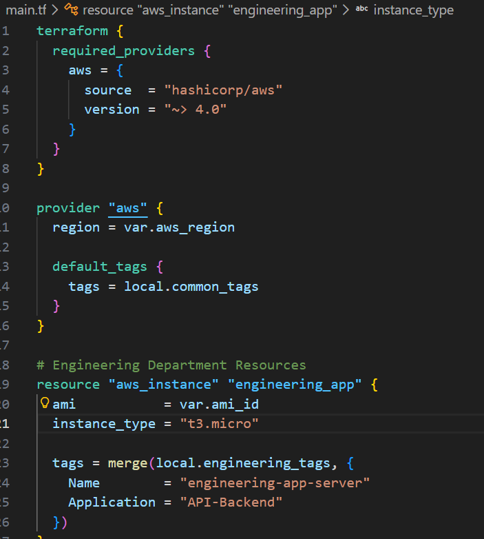
Step 3: Deploy Department-Specific Resources

Create main.tf with resources for each department:

terraform {
  required_providers {
    aws = {
      source  = "hashicorp/aws"
      version = "~> 4.0"
    }
  }
}

provider "aws" {
  region = var.aws_region
  
  default_tags {
    tags = local.common_tags
  }
}

# Engineering Department Resources
resource "aws_instance" "engineering_app" {
  ami           = var.ami_id
  instance_type = "t3.medium"
  
  tags = merge(local.engineering_tags, {
    Name        = "engineering-app-server"
    Application = "API-Backend"
  })
}

resource "aws_s3_bucket" "engineering_data" {
  bucket = "finops-engineering-data-${var.account_id}"
  
  tags = merge(local.engineering_tags, {
    Name     = "engineering-data-bucket"
    DataType = "Application-Logs"
  })
}

resource "aws_db_instance" "engineering_db" {
  identifier           = "engineering-postgres"
  engine              = "postgres"
  engine_version      = "15.3"
  instance_class      = "db.t3.micro"
  allocated_storage   = 20
  username            = "appowner"
  password            = var.db_password
  skip_final_snapshot = true
  
  tags = merge(local.engineering_tags, {
    Name        = "engineering-database"
    Application = "API-Backend"
  })
}

# Finance Department Resources
resource "aws_instance" "finance_reporting" {
  ami           = var.ami_id
  instance_type = "t3.small"
  
  tags = merge(local.finance_tags, {
    Name        = "finance-reporting-server"
    Application = "Financial-Reporting"
  })
}

resource "aws_s3_bucket" "finance_reports" {
  bucket = "finops-finance-reports-${var.account_id}"
  
  tags = merge(local.finance_tags, {
    Name     = "finance-reports-bucket"
    DataType = "Financial-Data"
  })
}

# Marketing Department Resources
resource "aws_instance" "marketing_web" {
  ami           = var.ami_id
  instance_type = "t3.small"
  
  tags = merge(local.marketing_tags, {
    Name        = "marketing-web-server"
    Application = "Campaign-Website"
  })
}

resource "aws_s3_bucket" "marketing_assets" {
  bucket = "finops-marketing-assets-${var.account_id}"
  
  tags = merge(local.marketing_tags, {
    Name     = "marketing-assets-bucket"
    DataType = "Media-Content"
  })
}

resource "aws_cloudfront_distribution" "marketing_cdn" {
  enabled = true
  
  origin {
    domain_name = aws_s3_bucket.marketing_assets.bucket_regional_domain_name
    origin_id   = "S3-marketing-assets"
  }
  
  default_cache_behavior {
    allowed_methods        = ["GET", "HEAD"]
    cached_methods         = ["GET", "HEAD"]
    target_origin_id       = "S3-marketing-assets"
    viewer_protocol_policy = "redirect-to-https"
    
    forwarded_values {
      query_string = false
      cookies {
        forward = "none"
      }
    }
  }
  
  restrictions {
    geo_restriction {
      restriction_type = "none"
    }
  }
  
  viewer_certificate {
    cloudfront_default_certificate = true
  }
  
  tags = merge(local.marketing_tags, {
    Name        = "marketing-cdn"
    Application = "Campaign-Website"
  })
}

Step 4: Create Variables File

Define variables.tf:

variable "aws_region" {
  description = "AWS region for resources"
  type        = string
  default     = "us-east-1"
}

variable "environment" {
  description = "Environment name"
  type        = string
  default     = "production"
}

variable "account_id" {
  description = "AWS Account ID"
  type        = string
}

variable "ami_id" {
  description = "AMI ID for EC2 instances"
  type        = string
}

variable "db_password" {
  description = "Database password"
  type        = string
  sensitive   = true
}

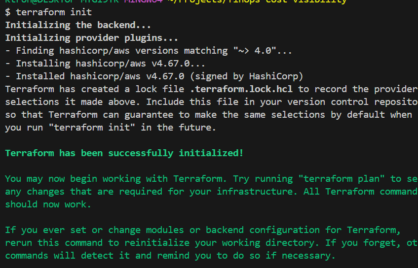
Step 5: Deploy the Infrastructure

# Initialize Terraform
terraform init

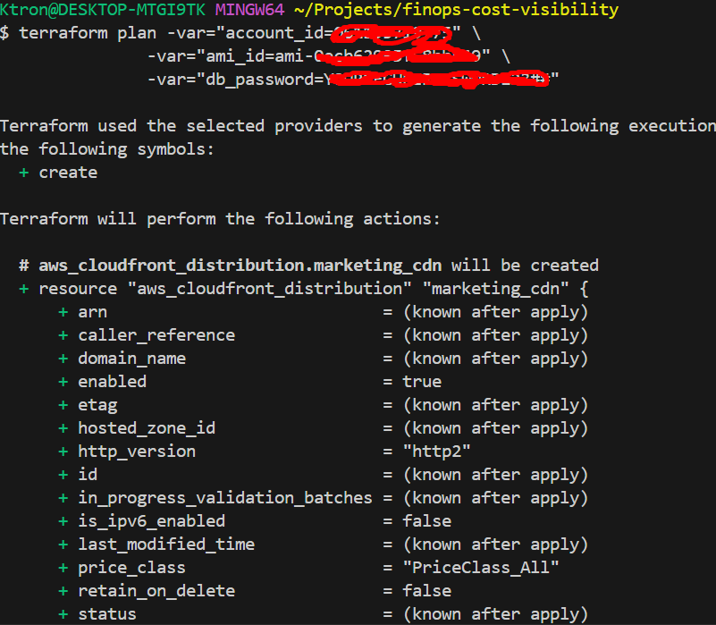
# Review the plan
terraform plan -var="account_id=YOUR_ACCOUNT_ID" \
               -var="ami_id=ami-XXXXXXXXX" \
               -var="db_password=YOUR_SECURE_PASSWORD"

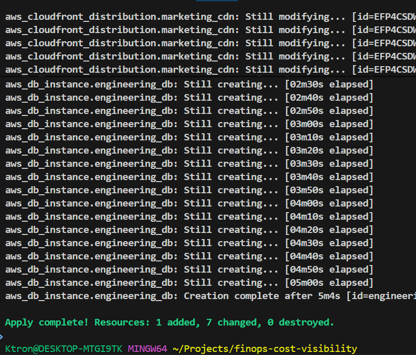
# Deploy resources
terraform apply -var="account_id=YOUR_ACCOUNT_ID" \
                -var="ami_id=ami-XXXXXXXXX" \
                -var="db_password=YOUR_SECURE_PASSWORD"

Step 6: Activate Cost Allocation Tags in AWS

1. Navigate to AWS Billing Console → Cost Allocation Tags
2. Activate the following user-defined tags:
   • Department
   • CostCenter
   • Owner
   • Application
   • Environment
   • Project

Note: Tags take 24 hours to appear in Cost Explorer after activation.

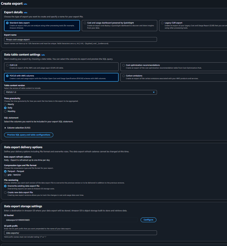
Setting Up AWS Data Exports

Step 1: Create Data Export via AWS Console

1. Navigate to Data Exports
   • Go to AWS Billing Console → Data Exports
   • Click “Create export”
2. Configure Export Settings
   • Export name: finops-cost-usage-export
   • Export type: Select “Standard data export”
   • Data refresh: Enable “Include resource IDs”
   • Time granularity: DAILY
3. Configure S3 Destination
   • S3 bucket: <ur-bucket-name>
   • S3 prefix: data-exports/
   • Compression: Parquet (best for Athena)
4. Review and Create
   • Review settings
   • Create export

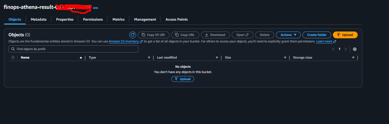
Set Up Athena

Create S3 Bucket for Athena Results

1. Navigate to S3
   • Create another bucket: finops-athena-results-YOUR_ACCOUNT_ID
   • Same region as your data exports bucket
   • Keep default settings

Create Athena Database

1. Navigate to Athena
   • Go to AWS Console → Athena
   • If first time, you’ll see a setup prompt
2. Set Query Result Location
   • Click “Settings” (or “Manage” → “Settings”)
   • Query result location: s3://finops-athena-results-YOUR_ACCOUNT_ID/queries/
   • Click “Save”
3. Create Database
   • In the query editor, run:

CREATE DATABASE IF NOT EXISTS finops_cost_data
COMMENT 'Database for FinOps cost and usage analysis';

• Click “Run”
• Verify database appears in left sidebar

Set Up AWS Glue Crawler

Why Glue Crawler? It automatically discovers the schema of your Data Export files and creates tables in Athena.

1. Navigate to AWS Glue
   • Go to AWS Console → AWS Glue
   • Click “Crawlers” in left menu
2. Create Crawler
   • Click “Create crawler”
   • Name: finops-cost-data-crawler
   • Click “Next”
3. Configure Data Source
   • Add data source: S3
   • S3 path: s3://finops-data-exports-YOUR_ACCOUNT_ID/data-exports/
   • Click “Add an S3 data source”
   • Click “Next”
4. Create IAM Role
   • Choose “Create new IAM role”
   • Role name: AWSGlueServiceRole-FinOps
   • Click “Next”
5. Set Output Database
   • Target database: Select finops_cost_data
   • Table name prefix: (leave blank or use cur_)
   • Click “Next”
6. Set Crawler Schedule
   • Frequency: Daily (or as needed)
   • Start time: Choose a time after your data export typically arrives (e.g., 8 AM)
   • Click “Next”
7. Review and Create
   • Review settings
   • Click “Create crawler”
8. Run Crawler Immediately
   • Select your crawler
   • Click “Run”
   • Wait for status to show “Succeeded” (may take 5-10 minutes)

Note: After the crawler runs successfully, you’ll see a new table in your finops_cost_data database!

4.4: Verify Table Creation

1. Go Back to Athena
   • Navigate to Athena console
   • Select database: finops_cost_data
   • You should see a table (likely named something like cost_and_usage_report)
2. Test Query
   • Run a simple test query:

SELECT * FROM cost_and_usage_report LIMIT 10;

If you see results, congratulations! Your setup is complete! 🎉

Step 5: Create Department-Specific Athena Views (Console)

Now let’s create SQL views for each department. In Athena query editor, run these queries one by one:

View 1: Engineering Department Costs

CREATE OR REPLACE VIEW engineering_costs AS
SELECT
    billing_period,
    regionname,
    servicename AS service,
    resourcetype AS resource_type,
    tags['user:Application'] AS application,
    chargecategory AS charge_type,
    COUNT(*) as line_items
FROM
    data
WHERE
    tags['user:Department'] = 'Engineering'
    AND chargecategory != 'Tax'
GROUP BY
    billing_period,
    regionname,
    servicename,
    resourcetype,
    tags['user:Application'],
    chargecategory
ORDER BY
    billing_period DESC,
    line_items DESC;

Click “Run” and you should see “Query successful” message.

View 2: Finance Department Costs

CREATE OR REPLACE VIEW finance_costs AS
SELECT
    billing_period,
    regionname,
    servicename AS service,
    resourcetype AS resource_type,
    tags['user:Application'] AS application,
    chargecategory AS charge_type,
    COUNT(*) as line_items
FROM
    data
WHERE
    tags['user:Department'] = 'Finance'
    AND chargecategory != 'Tax'
GROUP BY
    billing_period,
    regionname,
    servicename,
    resourcetype,
    tags['user:Application'],
    chargecategory
ORDER BY
    billing_period DESC,
    line_items DESC;

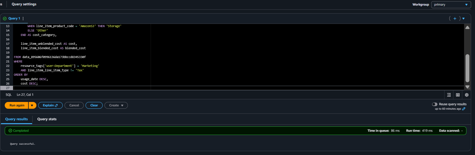
View 3: Marketing Department Costs

CREATE OR REPLACE VIEW marketing_costs AS
SELECT
    billing_period,
    regionname,
    servicename AS service,
    servicecategory AS cost_category,
    resourcetype AS resource_type,
    tags['user:Application'] AS application,
    chargecategory AS charge_type,
    COUNT(*) as line_items
FROM
    data
WHERE
    tags['user:Department'] = 'Marketing'
    AND chargecategory != 'Tax'
GROUP BY
    billing_period,
    regionname,
    servicename,
    servicecategory,
    resourcetype,
    tags['user:Application'],
    chargecategory
ORDER BY
    billing_period DESC,
    line_items DESC;

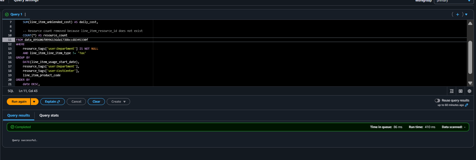
View 4: Executive Summary

CREATE OR REPLACE VIEW executive_summary AS
SELECT
    billing_period,
    tags['user:Department'] AS department,
    tags['user:CostCenter'] AS cost_center,
    servicename AS service,
    servicecategory AS service_category,
    regionname,
    COUNT(*) AS total_line_items,
    COUNT(DISTINCT resourcetype) AS unique_resources
FROM 
    data
WHERE
    tags['user:Department'] IS NOT NULL
    AND chargecategory != 'Tax'
GROUP BY
    billing_period,
    tags['user:Department'],
    tags['user:CostCenter'],
    servicename,
    servicecategory,
    regionname
ORDER BY
    billing_period DESC,
    total_line_items DESC;

Verify Views Created:

• In Athena left sidebar, expand “Views” under your database
• You should see all 4 views listed

Test Your Views with Sample Queries

Now let’s query each view to see department-specific data:

Test Engineering View

SELECT 
    billing_period,
    regionname,
    service,
    application,
    charge_type,
    SUM(line_items) as total_items
FROM engineering_costs
GROUP BY 
    billing_period,
    regionname,
    service,
    application,
    charge_type
ORDER BY 
    billing_period DESC,
    total_items DESC;

Test Finance View

SELECT 
    billing_period,
    service,
    application,
    SUM(line_items) as total_items
FROM finance_costs
GROUP BY 
    billing_period,
    service,
    application
ORDER BY 
    total_items DESC;

Test Marketing View

SELECT 
    billing_period,
    service,
    cost_category,
    application,
    SUM(line_items) as total_items
FROM marketing_costs
GROUP BY 
    billing_period,
    service,
    cost_category,
    application
ORDER BY 
    total_items DESC;

Test Executive Summary

SELECT 
    billing_period,
    department,
    cost_center,
    service,
    SUM(total_line_items) as total_items,
    SUM(unique_resources) as total_resources
FROM executive_summary
GROUP BY 
    billing_period,
    department,
    cost_center,
    service
ORDER BY 
    billing_period DESC,
    total_items DESC;

QuickSight Initial Setup

Step 1: Sign Up for Amazon QuickSight

1. Navigate to QuickSight
   • Go to AWS Console → Search “QuickSight”
   • Click “Sign up for QuickSight” (if first time)
2. Choose Edition
   • Select Enterprise Edition (recommended for production)
   • Or Standard Edition (for testing)
   • Click “Continue”
3. Configure QuickSight Account
   • QuickSight account name: finops-analytics
   • Notification email: Your email address
   • QuickSight region: Same as your Athena region
   • Click “Finish”
4. Grant Permissions
   • Enable: Amazon Athena ✓
   • Enable: Amazon S3 ✓
   • Click “Choose S3 buckets”
   • Select:
     • finops-data-exports-YOUR_ACCOUNT_ID ✓
     • finops-athena-results-YOUR_ACCOUNT_ID ✓
   • Click “Finish”

Part 2: Connect QuickSight to Athena

Step 1: Create Athena Data Source

1. Go to Datasets
   • In QuickSight console, click “Datasets” in left menu
   • Click “New dataset”
2. Select Athena
   • Click on “Athena” card
   • Data source name: finops-athena-source
   • Athena workgroup: primary (or your custom workgroup)
   • Click “Create data source”
3. Choose Database and Table
   • Catalog: AwsDataCatalog
   • Database: finops_cost_data
   • Tables: Select engineering_costs first
   • Click “Select”
4. Configure Data Import
   • Choose “Directly query your data” (SPICE can be enabled later for better performance)
   • Click “Visualize”

Part 3: Create Engineering Department Dashboard

Step 1: Set Up Engineering Dataset

1. Edit Dataset (if needed)
   • In QuickSight, go to “Datasets”
   • Click on engineering_costs dataset
   • Click “Edit dataset”
2. Add Calculated Fields (Optional)
   • Click “Add calculated field”
   • Month Name:

     formatDate(parseDate(billing_period, "yyyy-MM"), "MMM yyyy")

• Click “Save”

Step 2: Build Engineering Dashboard

1. Create Analysis
   • From Datasets, click engineering_costs
   • Click “Create analysis”
   • Analysis name: Engineering Cost Analysis
2. Visual 1: Costs by Service (Donut Chart)
   • Click “Add” → “Add visual”
   • Visual type: Donut chart
   • Value: line_items (Sum)
   • Group by: service
   • Title: “Cost Distribution by Service”
3. Visual 2: Costs Over Time (Line Chart)
   • Click “Add” → “Add visual”
   • Visual type: Line chart
   • X-axis: billing_period
   • Value: line_items (Sum)
   • Color: service
   • Title: “Monthly Cost Trend by Service”
4. Visual 3: Costs by Region (Bar Chart)
   • Click “Add” → “Add visual”
   • Visual type: Horizontal bar chart
   • Y-axis: regionname
   • Value: line_items (Sum)
   • Title: “Costs by AWS Region”
5. Visual 4: Costs by Application (Table)
   • Click “Add” → “Add visual”
   • Visual type: Table
   • Rows:
     • application
     • service
     • resource_type
   • Values: line_items (Sum)
   • Title: “Detailed Costs by Application”
6. Visual 5: Charge Type Breakdown (Stacked Bar)
   • Click “Add” → “Add visual”
   • Visual type: Stacked bar chart
   • X-axis: billing_period
   • Value: line_items (Sum)
   • Group/Color: charge_type
   • Title: “Cost Breakdown by Charge Type”
7. Add Filters
   • Click “Filter” in left panel
   • Add filter: billing_period
     • Filter type: Time range
     • Select last 6 months
   • Add filter: service
     • Filter type: Multi-select
     • Make it a control (so users can select)
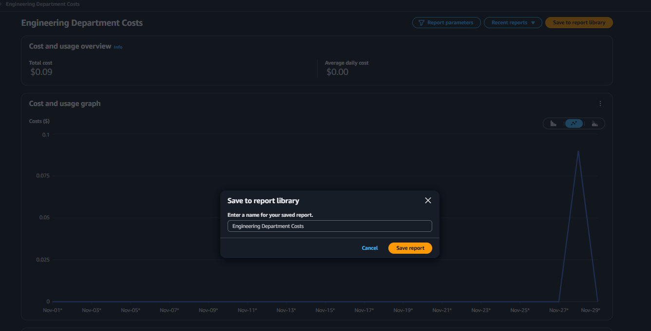
8. Publish Dashboard
   • Click “Share” → “Publish dashboard”
   • Dashboard name: Engineering Department Costs
   • Click “Publish dashboard”

Part 2: Creating Department-Specific Dashboards

Manual Dashboard Creation in AWS Cost Explorer

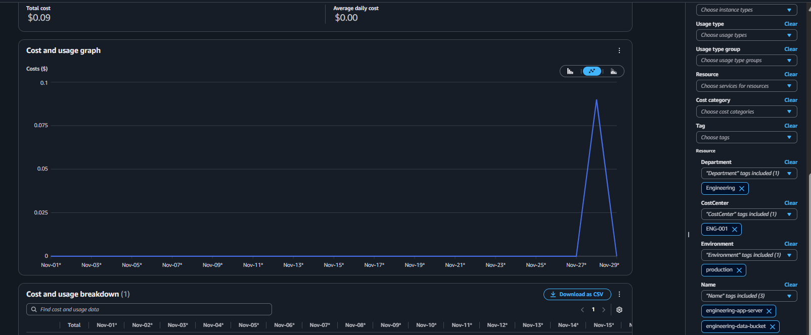
Dashboard 1: Engineering Department View

1. Navigate to Cost Explorer
   • Go to Cost Management → Cost Explorer
2. Create Engineering Cost Report
   • On the right side, you have:
   • Time section
   • Group by
   • Filters
   • Chart type buttons
   • Save to report library
3. Set Your Time Range
4. On the right panel:
5. Time → Standard
6. Date Range: choose
   Last 3 Months
7. Granularity:
   Change to Daily
   (Important: this defaults to Monthly)
8. Apply Filters
   • Filter by Tag: Department = “Engineering”
   • Group by: Service
9. Customize Visualization
   • Chart type: Stacked bar chart
   • Show: Costs
   • Additional grouping: Add “Application” tag
10. Add Cost Breakdown Section
    • Create another chart grouped by: CostCenter, Application
    • This shows cost distribution across engineering projects
11. Save the Report
    • Click “Save as” → “Save report”
    • Add to dashboard

Dashboard 2: Finance Department View

1. Create Finance Cost Report
   • Name: “Finance Department Costs”
   • Filter by Tag: Department = “Finance”
   • Group by: Service and Resource
2. Add Budget Tracking
   • Include budget vs. actual spending
   • Set up anomaly detection alerts
3. Cost Trend Analysis
   • Add month-over-month comparison
   • Include forecast for next 30 days

Dashboard 3: Marketing Department View

1. Create Marketing Cost Report
   • Name: “Marketing Department Costs”
   • Filter by Tag: Department = “Marketing”
   • Group by: Service (focus on CloudFront, S3)
2. Campaign-Specific View
   • Group by “Application” tag to see per-campaign costs
   • Add data transfer costs analysis
3. ROI Metrics
   • Include custom metrics for cost per campaign
   • Add notes section for campaign performance

Creating a Unified Executive Dashboard

1. Multi-Department Overview
   • Name: “Executive Cost Overview”
   • Group by: Department
   • Time period: Current month vs. previous month
2. Key Metrics to Include
   • Total spend by department
   • Top 5 cost-driving services
   • Month-over-month growth rate
   • Budget utilization percentage
3. Cost Anomaly Section
   • Enable anomaly detection
   • Set thresholds for alerts
   • Review daily spikes or unusual patterns

Next Steps: The Optimize Phase

Now that you have visibility (Inform), the next phase is Optimize:

1. Identify Waste: Use your dashboards to find idle resources
2. Right-Size: Match instance types to actual usage
3. Use Committed Use Discounts: Reserved Instances and Savings Plans
4. Automate Schedules: Stop dev/test resources after hours
5. Storage Optimization: Delete old snapshots, use lifecycle policies

Conclusion

We now have a production-ready FinOps cost visibility platform! Here’s what we accomplished:

✅ Deployed tagged infrastructure with Terraform
✅ Created three department-specific dashboards
✅ Set up automated daily and weekly reports
✅ Configured budget alerts and anomaly detection
✅ Built a foundation for ongoing cost optimization

The Inform phase of FinOps is complete. You have the visibility needed to make data-driven decisions about your cloud spending.